The analysis of electromechanical dynamics relies significantly on the generator rotor swing following a fault in the grid. To analyze electromechanical dynamics, it can be assumed that the shaft of the generating unit is rigid, and the rotor swing can be described as:

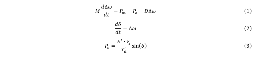
where the time derivative of the rotor angle dδ/dt = Δω = ω − ω_s is the rotor speed deviation in electrical radians per second (rad/s), D is the damping coefficient,  E’ is transient internal emf, V_s is infinite busbar voltage, x_d’ is d-axis transient reactance between generator and the infinite busbar,  is the power (or rotor) angle with respect to the infinite busbar, and P_m and P_e are the mechanical and electrical power, respectively. The coefficient M is defined as:

Where H is the inertia constant, S_n is the generator nominal power.

The response of a system to a significant disturbance, such as a short circuit or line tripping, is very dramatic from a stability standpoint. When such a fault happens, substantial currents and torques are generated, and swift action is often necessary to preserve system stability. This challenge is commonly referred to as the issue of large-disturbance stability.

Four distinct types of short circuits, namely single-phase short circuit, phase-to-phase short circuit, phase-to-phase-to-earth short circuit, and three-phase short circuit, are examined on the single-machine-infinite-busbar (SMIB) system depicted in Figure 1. The short circuit occurs at the beginning of the line.

Figure 1. Schematic diagram of the SMIB system

The initial step involves determining the power-angle curve P_{e_pre} for the normal grid. Assuming E’ and V_s remain constant, the focus is on finding the equivalent system reactance  as shown in Figure 2.

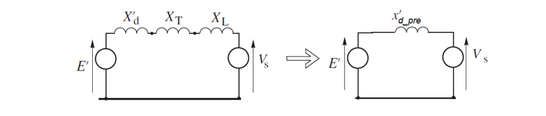
Figure 2. Equivalent circuit for the pre-fault state

The second step involves determining the power-angle curve P_{e_fault} for the fault state. Assuming E’ and V_s remain constant, the focus is on finding the equivalent system reactance during fault () according to Figure 3.

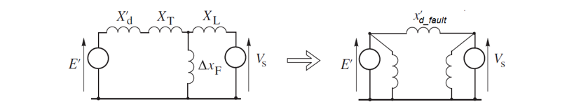
Figure 3. Equivalent circuit for the fault state

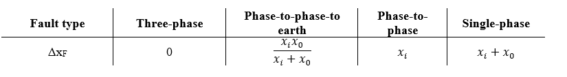
Utilizing symmetrical components enables the representation of any type of fault in the positive-sequence network by introducing a fault shunt reactance (Δx_F) connected between the point of the fault and the neutral, as illustrated in Figure 3. The value of Δx_F is contingent on the type of fault and is provided in Table 1, where x_i and x₀ are the negative and zero-sequence Thévenin equivalent reactances observed from the fault terminals.

can be calculated using star-delta transformation as shown in Figure 3:

The power-angle curve P_{e_fault} for the fault state is:

Finally, the last step is to determine the power-angle curve P_{e_post} post-fault, which, in the case of this grid, is the same as the power-angle curve for the normal grid (pre-fault) i.e.:

To assess rotor-angle stability during the fault, it’s essential to analyze the yellow (P_acc) and blue (P_dcc) areas in the interactive graph below. For stable operation, the deceleration (blue) area must be larger than the acceleration (yellow) area. The sizes of both areas primarily depend on the time it takes to clear the fault, i.e., the angle delta_cl when the fault is cleared.